
Best for
- Processing ELISA plate data with standard curve fitting (4PL)
- Quantifying IHC staining intensity (H-score, positive pixel percentage)
- Analyzing ATAC-seq peaks and differential chromatin accessibility
synthetic-sciences/openscience/backend/cli/skills/biology/immunology-assays/SKILL.md
Computational analysis of immunology experimental data. ATAC-seq differential accessibility, immune cell tracking from microscopy, ELISA data processing with 4-parameter logistic fitting, immunohistochemistry quantification, antibody titer analysis, and cell cycle phase duration estimation. For flow cytometry use flow-cytometry-analysis; for scRNA-seq use scanpy.
Decision brief
Computational analysis of immunology experimental data. ATAC-seq differential accessibility, immune cell tracking from microscopy, ELISA data processing with 4-parameter logistic fitting, immunohistochemistry quantification, antibody titer analysis, and cell cycle phase duration estimation.
In this controlled same-task single run, enabling immunology-assays changed the output from 2201 non-whitespace characters and 13 headings to 2509 characters and 12 headings. Matches among 8 signals extracted from the pinned source changed from 1 to 1. Both actual outputs are shown; this is a structural observation, not a quality score or a universal performance claim.
Create a design direction and implementation handoff for a developer tool that compares two API responses. Prioritize the repeated user workflow and responsive behavior. The deliverable must specifically reflect this user intent: Computational analysis of immunology experimental data. ATAC-seq differential accessibility, immune cell tracking from microscopy, ELISA data processing with 4-parameter logistic fitting, immunohistochemistry quantification, antibody titer analysis, and cell cycle phase duration estimation. For flow cytometry use flow-cytometry-analysis; for scRNA-seq use scanpy.
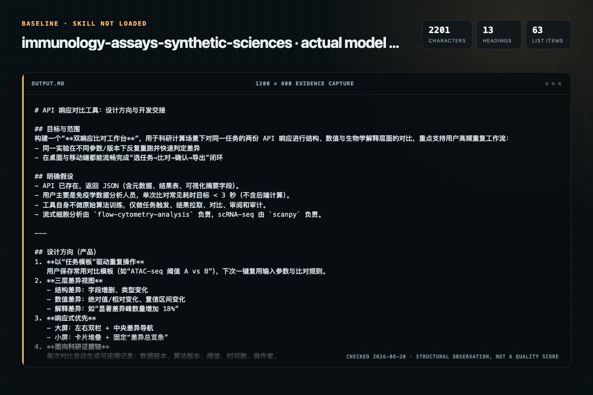
Baseline: 2201 non-whitespace characters, 13 headings, and 63 list items.
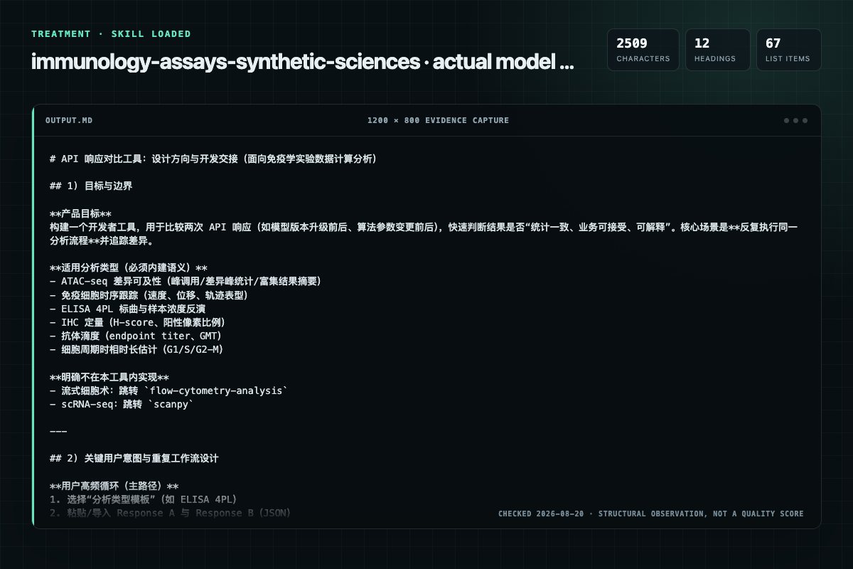
With Skill: 2509 non-whitespace characters, 12 headings, and 67 list items.
| Observation | Without Skill | With Skill |
|---|---|---|
| Source-signal coverage | 1/8: analysis | 1/8: analysis |
| Output structure | 2201 chars · 13 headings · 63 list items · 0 code blocks | 2509 chars · 12 headings · 67 list items · 1 code blocks |
| Verification and caution signals | 3 verification signals · 3 risk/limitation signals | 7 verification signals · 2 risk/limitation signals |
Use the immunology-assays Skill pinned at 0e1e42e75212 for my task. Follow its source-specific constraints around `immunology-assays`, `immunology`, `assays`, `experimental`, then return the finished deliverable with explicit assumptions, verification, failure conditions, and limits. Do not treat the Skill text as a factual source or claim that a single demonstration proves universal performance.
Compatibility matrix
| Platform | Status | Evidence | What to check |
|---|---|---|---|
| Codex | Not declared | No explicit evidence | Portability before use |
| Claude Code | Not declared | No explicit evidence | Portability before use |
| Cursor | Not declared | No explicit evidence | Portability before use |
| Gemini CLI | Not declared | No explicit evidence | Portability before use |
Installation
The source command is displayed only when detected. A safe inspection prompt is always available so your agent can explain every action before execution.
npx skills add https://github.com/synthetic-sciences/openscience --skill "backend/cli/skills/biology/immunology-assays"Inspect the Agent Skill "immunology-assays" from https://github.com/synthetic-sciences/openscience/blob/d7129109cc959e2bbbfee84bba019e4e722221da/backend/cli/skills/biology/immunology-assays/SKILL.md at commit d7129109cc959e2bbbfee84bba019e4e722221da. List every install step, command, network request, credential, file read/write, external action, and rollback step. Explain whether it fits my task. Do not install or execute anything until I approve.
Workflow
python import numpy as np from scipy.optimize import curvefit
Estimate phase durations from dual-nucleoside pulse labeling.
Review the “Workflow 1: Process ELISA Plate Data with 4PL Standard Curve” section in the pinned source before continuing.
Review the “Workflow 2: Quantify IHC Staining Intensity (H-Score)” section in the pinned source before continuing.
Review the “Workflow 3: ATAC-seq Peak Calling and Differential Accessibility” section in the pinned source before continuing.
Permission review
No configured static risk pattern was detected
This is not proof of safety. Runtime behavior, indirect dependencies, and hidden external systems are outside the static scan.
Evidence record
| Signal | Value | Evidence type | Meaning |
|---|---|---|---|
| Quality score | 93/100 | Computed | Documentation, specificity, maintenance, and trust rules |
| Repository stars | 3,337 | Source | Repository attention, not individual Skill quality |
| Compatibility | 0 platforms | Source | Declared in the catalog source record |
| Usage guide | tested outcome page | Tested | Generated or reviewed according to the visible evidence level |
Pinned source
Immunology Assays provides computational tools for analyzing data from common immunology experiments. This skill covers ATAC-seq differential accessibility analysis (MACS2 peak calling, motif enrichment), ELISA data processing with 4-parameter logistic standard curve fitting, immune cell tracking from time-lapse microscopy, immunohistochemistry (IHC) quantification with H-score calculation, antibody titer determination from serial dilution ELISA, cell cycle phase duration estimation from dual-nucleoside labeling, and multiplex cytokine assay data processing.
Related Skills: For flow cytometry analysis use flow-cytometry-analysis. For single-cell RNA-seq use scanpy. For bioimage analysis use bioimage-analysis.
uv pip install scipy scikit-image opencv-python numpy pandas matplotlib
For ATAC-seq (optional):
# conda install -c bioconda macs2 homer
import numpy as np
from scipy.optimize import curve_fit

# 4-Parameter Logistic (4PL) for ELISA standard curve
def four_pl(x, a, b, c, d):
    """a=min, b=Hill slope, c=EC50, d=max"""
    return d + (a - d) / (1 + (x / c) ** b)

# Standard curve data
concentrations = np.array([0, 15.6, 31.25, 62.5, 125, 250, 500, 1000])
od_values = np.array([0.05, 0.12, 0.22, 0.45, 0.82, 1.35, 1.85, 2.15])

popt, pcov = curve_fit(four_pl, concentrations[1:], od_values[1:],
                       p0=[0.05, 1.0, 200, 2.2], maxfev=10000)
print(f"EC50: {popt[2]:.1f} pg/mL")
print(f"Dynamic range: {popt[0]:.3f} - {popt[3]:.3f} OD")
Peak calling and differential accessibility.
import subprocess
import pandas as pd

def run_macs2_atacseq(bam_path, output_prefix, genome_size='hs'):
    """Call ATAC-seq peaks with MACS2."""
    cmd = [
        'macs2', 'callpeak',
        '-t', bam_path,
        '-f', 'BAMPE',           # Paired-end
        '-g', genome_size,
        '--nomodel',
        '--shift', '-100',
        '--extsize', '200',
        '--broad',               # Broad peaks for open chromatin
        '-n', output_prefix,
        '--outdir', 'macs2_output'
    ]
    result = subprocess.run(cmd, capture_output=True, text=True)
    if result.returncode != 0:
        raise RuntimeError(f"MACS2 failed: {result.stderr}")
    return f'macs2_output/{output_prefix}_peaks.broadPeak'

def parse_broadpeak(peak_file):
    """Parse MACS2 broadPeak output."""
    cols = ['chrom', 'start', 'end', 'name', 'score', 'strand',
            'signal', 'pvalue', 'qvalue']
    df = pd.read_csv(peak_file, sep='\t', header=None, names=cols)
    print(f"Total peaks: {len(df)}")
    print(f"Mean peak width: {(df['end'] - df['start']).mean():.0f} bp")
    return df

def differential_accessibility(count_matrix, conditions, padj_threshold=0.05):
    """DESeq2-style differential accessibility from peak count matrix.

    Args:
        count_matrix: peaks x samples DataFrame (integer counts)
        conditions: list of condition labels per sample
    """
    from scipy.stats import mannwhitneyu
    from statsmodels.stats.multitest import multipletests

    results = []
    groups = list(set(conditions))
    g1_idx = [i for i, c in enumerate(conditions) if c == groups[0]]
    g2_idx = [i for i, c in enumerate(conditions) if c == groups[1]]

    for peak in count_matrix.index:
        vals1 = count_matrix.loc[peak].iloc[g1_idx].values
        vals2 = count_matrix.loc[peak].iloc[g2_idx].values

        fc = (vals2.mean() + 1) / (vals1.mean() + 1)
        log2fc = np.log2(fc)

        stat, pval = mannwhitneyu(vals1, vals2, alternative='two-sided')
        results.append({'peak': peak, 'log2FC': log2fc, 'pvalue': pval})

    df = pd.DataFrame(results)
    _, df['padj'], _, _ = multipletests(df['pvalue'], method='fdr_bh')

    sig = df[df['padj'] < padj_threshold]
    print(f"Significant DA peaks: {len(sig)} / {len(df)}")
    print(f"  More accessible: {(sig['log2FC'] > 0).sum()}")
    print(f"  Less accessible: {(sig['log2FC'] < 0).sum()}")
    return df

def run_homer_motif(peak_bed, genome, output_dir):
    """Run HOMER motif enrichment on peaks."""
    cmd = [
        'findMotifsGenome.pl', peak_bed, genome, output_dir,
        '-size', '200', '-mask', '-p', '4'
    ]
    subprocess.run(cmd, capture_output=True, text=True, check=True)
    return output_dir
4-parameter logistic standard curve fitting and unknown interpolation.
import numpy as np
from scipy.optimize import curve_fit
import pandas as pd

def four_pl(x, a, b, c, d):
    """4-Parameter Logistic curve.
    a = minimum asymptote, b = Hill slope, c = EC50, d = maximum asymptote"""
    return d + (a - d) / (1 + (x / c) ** b)

def inverse_four_pl(y, a, b, c, d):
    """Inverse 4PL to interpolate concentration from OD."""
    return c * ((a - d) / (y - d) - 1) ** (1 / b)

def process_elisa_plate(standards, unknowns, blank_od=None):
    """Process ELISA plate with 4PL standard curve.

    Args:
        standards: dict of concentration -> list of OD replicates
        unknowns: dict of sample_name -> list of OD replicates
        blank_od: blank well OD (subtracted from all values)
    """
    # Prepare standard curve data
    conc_list, od_list = [], []
    for conc, ods in sorted(standards.items()):
        for od in ods:
            if conc > 0:  # Skip zero for fitting
                conc_list.append(conc)
                od_list.append(od - (blank_od or 0))

    conc_arr = np.array(conc_list)
    od_arr = np.array(od_list)

    # Fit 4PL
    p0 = [min(od_arr), 1.0, np.median(conc_arr), max(od_arr)]
    popt, pcov = curve_fit(four_pl, conc_arr, od_arr, p0=p0, maxfev=10000)
    a, b, c, d = popt

    # R-squared
    predicted = four_pl(conc_arr, *popt)
    ss_res = np.sum((od_arr - predicted) ** 2)
    ss_tot = np.sum((od_arr - np.mean(od_arr)) ** 2)
    r_squared = 1 - ss_res / ss_tot

    # Detection limits
    lod = inverse_four_pl(a + 2 * np.std(od_arr[:3]), *popt) if a + 2 * np.std(od_arr[:3]) < d else None

    print(f"4PL fit: R² = {r_squared:.4f}")
    print(f"EC50: {c:.2f}")
    print(f"Dynamic range: {a:.3f} - {d:.3f} OD")
    if lod:
        print(f"LOD: {lod:.2f}")

    # Interpolate unknowns
    results = []
    for name, ods in unknowns.items():
        od_corrected = [od - (blank_od or 0) for od in ods]
        concentrations = []
        for od in od_corrected:
            if a < od < d:  # Within curve range
                conc = inverse_four_pl(od, *popt)
                concentrations.append(conc)
            else:
                concentrations.append(np.nan)

        results.append({
            'sample': name,
            'mean_od': np.mean(od_corrected),
            'mean_conc': np.nanmean(concentrations),
            'std_conc': np.nanstd(concentrations),
            'n': len(concentrations),
            'in_range': sum(~np.isnan(c) for c in concentrations)
        })

    return pd.DataFrame(results), popt, r_squared

# Example
standards = {
    0: [0.05, 0.06], 15.6: [0.11, 0.13], 31.25: [0.21, 0.23],
    62.5: [0.44, 0.46], 125: [0.80, 0.84], 250: [1.32, 1.38],
    500: [1.82, 1.88], 1000: [2.12, 2.18]
}
unknowns = {
    'Patient_1': [0.95, 0.98], 'Patient_2': [0.35, 0.38],
    'Patient_3': [1.55, 1.60], 'Control': [0.08, 0.09]
}

results, params, r2 = process_elisa_plate(standards, unknowns, blank_od=0.05)
print(results[['sample', 'mean_conc', 'std_conc']])
Track immune cells in time-lapse microscopy.
import numpy as np
import pandas as pd

def track_immune_cells(tracks_df, pixel_size_um=0.65, frame_interval_min=1):
    """Analyze immune cell migration from tracking data.

    Args:
        tracks_df: DataFrame with columns [particle, frame, x, y]
        pixel_size_um: microns per pixel
        frame_interval_min: minutes between frames
    """
    results = []

    for pid, track in tracks_df.groupby('particle'):
        track = track.sort_values('frame')
        x = track['x'].values * pixel_size_um
        y = track['y'].values * pixel_size_um
        t = track['frame'].values * frame_interval_min

        # Instantaneous velocity
        dx = np.diff(x)
        dy = np.diff(y)
        dt = np.diff(t)
        speeds = np.sqrt(dx**2 + dy**2) / dt

        # Displacement (start to end)
        displacement = np.sqrt((x[-1] - x[0])**2 + (y[-1] - y[0])**2)

        # Total path length
        path_length = np.sum(np.sqrt(dx**2 + dy**2))

        # Confinement ratio (displacement / path_length)
        confinement = displacement / path_length if path_length > 0 else 0

        # Mean squared displacement
        msd_values = []
        for lag in range(1, min(len(x), 20)):
            displacements = (x[lag:] - x[:-lag])**2 + (y[lag:] - y[:-lag])**2
            msd_values.append(np.mean(displacements))

        results.append({
            'particle': pid,
            'mean_speed': np.mean(speeds),
            'max_speed': np.max(speeds),
            'displacement': displacement,
            'path_length': path_length,
            'confinement_ratio': confinement,
            'duration_min': t[-1] - t[0],
            'n_frames': len(track)
        })

    df = pd.DataFrame(results)

    # Classify migratory phenotype
    df['phenotype'] = 'confined'
    df.loc[df['confinement_ratio'] > 0.5, 'phenotype'] = 'directed'
    df.loc[(df['confinement_ratio'] > 0.2) & (df['confinement_ratio'] <= 0.5), 'phenotype'] = 'random_walk'

    print(f"Tracked {len(df)} cells")
    print(f"Mean speed: {df['mean_speed'].mean():.2f} um/min")
    print(f"Phenotypes:\n{df['phenotype'].value_counts()}")
    return df
Quantify immunohistochemistry staining intensity.
import numpy as np
from skimage.color import rgb2hed
import skimage.io

def quantify_ihc(image_path, method='h_score'):
    """Quantify IHC staining using color deconvolution.

    Separates DAB (brown) from hematoxylin (blue) using
    Ruifrok & Johnston color deconvolution.
    """
    image = skimage.io.imread(image_path)

    # Color deconvolution: RGB → HED (Hematoxylin, Eosin, DAB)
    hed = rgb2hed(image)
    dab_channel = hed[:, :, 2]  # DAB is channel 2
    hematoxylin = hed[:, :, 0]

    # Threshold to identify tissue
    tissue_mask = hematoxylin > 0.05

    # DAB intensity classification for H-score
    dab_tissue = dab_channel[tissue_mask]

    # Classify: negative (0), weak (1+), moderate (2+), strong (3+)
    negative = (dab_tissue < 0.1).sum()
    weak = ((dab_tissue >= 0.1) & (dab_tissue < 0.2)).sum()
    moderate = ((dab_tissue >= 0.2) & (dab_tissue < 0.4)).sum()
    strong = (dab_tissue >= 0.4).sum()
    total = len(dab_tissue)

    # H-score: 1*(% weak) + 2*(% moderate) + 3*(% strong)
    h_score = (1 * weak + 2 * moderate + 3 * strong) / total * 100

    # Positive pixel percentage
    positive_pct = 100 * (weak + moderate + strong) / total

    print(f"H-score: {h_score:.1f} (range 0-300)")
    print(f"Positive pixels: {positive_pct:.1f}%")
    print(f"  Weak (1+): {100*weak/total:.1f}%")
    print(f"  Moderate (2+): {100*moderate/total:.1f}%")
    print(f"  Strong (3+): {100*strong/total:.1f}%")

    return {
        'h_score': h_score,
        'positive_pct': positive_pct,
        'negative_pct': 100 * negative / total,
        'weak_pct': 100 * weak / total,
        'moderate_pct': 100 * moderate / total,
        'strong_pct': 100 * strong / total
    }
Determine endpoint titers from serial dilution ELISA.
import numpy as np
from scipy import stats

def calculate_endpoint_titer(dilutions, od_values, cutoff_method='mean_plus_3sd',
                              negative_ods=None):
    """Determine endpoint antibody titer from serial dilution ELISA.

    Args:
        dilutions: list of dilution factors (e.g., [100, 200, 400, ...])
        od_values: list of OD values at each dilution
        negative_ods: list of negative control OD values
    """
    if negative_ods is None:
        cutoff = 0.1  # Default cutoff
    elif cutoff_method == 'mean_plus_3sd':
        cutoff = np.mean(negative_ods) + 3 * np.std(negative_ods)
    elif cutoff_method == 'mean_plus_2sd':
        cutoff = np.mean(negative_ods) + 2 * np.std(negative_ods)
    else:
        cutoff = 0.1

    # Find last dilution above cutoff
    endpoint = None
    for dil, od in zip(dilutions, od_values):
        if od > cutoff:
            endpoint = dil

    if endpoint is None:
        return {'titer': '<' + str(min(dilutions)), 'cutoff': cutoff}

    return {
        'titer': endpoint,
        'log2_titer': np.log2(endpoint),
        'cutoff': cutoff
    }

def geometric_mean_titer(titers):
    """Calculate geometric mean titer from multiple samples."""
    log_titers = np.log2([t for t in titers if t > 0])
    gmt = 2 ** np.mean(log_titers)
    ci = stats.t.interval(0.95, df=len(log_titers)-1,
                          loc=np.mean(log_titers),
                          scale=stats.sem(log_titers))
    return {
        'gmt': gmt,
        'ci_lower': 2 ** ci[0],
        'ci_upper': 2 ** ci[1],
        'n': len(log_titers)
    }

# Example
dilutions = [100, 200, 400, 800, 1600, 3200, 6400, 12800]
sample_ods = [2.1, 1.8, 1.4, 0.9, 0.45, 0.18, 0.08, 0.05]
neg_ods = [0.06, 0.05, 0.07, 0.04]

result = calculate_endpoint_titer(dilutions, sample_ods, negative_ods=neg_ods)
print(f"Endpoint titer: 1:{result['titer']}")
print(f"Cutoff OD: {result['cutoff']:.3f}")
Estimate phase durations from dual-nucleoside pulse labeling.
import numpy as np

def estimate_phase_durations(labeled_fractions, pulse_interval_hours,
                              total_cycle_time=None):
    """Estimate cell cycle phase durations from dual-nucleoside labeling.

    Args:
        labeled_fractions: dict of timepoints -> fraction labeled
        pulse_interval_hours: time between pulses
        total_cycle_time: if known, constrains the estimates
    """
    times = sorted(labeled_fractions.keys())
    fractions = [labeled_fractions[t] for t in times]

    # S-phase duration estimate: fraction labeled at first timepoint * total cycle time
    # If total cycle time unknown, estimate from growth rate
    if total_cycle_time is None:
        # Assume exponential growth, estimate from labeling kinetics
        # Rate of increase in labeled fraction approximates 1/Tc
        if len(fractions) > 1:
            rate = (fractions[-1] - fractions[0]) / (times[-1] - times[0])
            total_cycle_time = 1 / rate if rate > 0 else 24
        else:
            total_cycle_time = 24  # Default

    s_phase = fractions[0] * total_cycle_time
    g2m_phase = pulse_interval_hours  # Time for labeled cells to reach mitosis

    # G1 = total - S - G2/M
    g1_phase = total_cycle_time - s_phase - g2m_phase
    g1_phase = max(g1_phase, 0)

    return {
        'total_cycle': total_cycle_time,
        'G1': g1_phase,
        'S': s_phase,
        'G2_M': g2m_phase
    }
Process multiplex cytokine assay data.
import numpy as np
import pandas as pd
from scipy.optimize import curve_fit

def process_multiplex_cytokines(plate_data, analytes, standard_curves):
    """Process multiplex cytokine assay (Luminex/MSD) data.

    Args:
        plate_data: DataFrame with well, sample, analyte, MFI columns
        analytes: list of analyte names
        standard_curves: dict of analyte -> (concentrations, MFI_values)
    """
    def five_pl(x, a, b, c, d, g):
        return d + (a - d) / (1 + (x / c) ** b) ** g

    results = []
    for analyte in analytes:
        # Fit standard curve
        conc, mfi = standard_curves[analyte]
        try:
            popt, _ = curve_fit(five_pl, conc[conc > 0], mfi[conc > 0],
                               p0=[min(mfi), 1, np.median(conc), max(mfi), 1],
                               maxfev=10000)
        except RuntimeError:
            # Fall back to 4PL
            popt = None

        # Interpolate unknowns
        analyte_data = plate_data[plate_data['analyte'] == analyte]
        for _, row in analyte_data.iterrows():
            if popt is not None:
                # Inverse 5PL
                try:
                    from scipy.optimize import brentq
                    conc_val = brentq(lambda x: five_pl(x, *popt) - row['MFI'],
                                     0.01, 100000)
                except ValueError:
                    conc_val = np.nan
            else:
                conc_val = np.nan

            results.append({
                'sample': row['sample'],
                'analyte': analyte,
                'MFI': row['MFI'],
                'concentration': conc_val
            })

    return pd.DataFrame(results)
standards = {0: [0.05], 15.6: [0.12, 0.13], 31.25: [0.22, 0.24],
             62.5: [0.45, 0.47], 125: [0.82, 0.85], 250: [1.35, 1.38],
             500: [1.85, 1.88], 1000: [2.15, 2.18]}
unknowns = {'Sample_A': [0.68, 0.72], 'Sample_B': [1.45, 1.50]}
results, params, r2 = process_elisa_plate(standards, unknowns, blank_od=0.05)
print(results)
result = quantify_ihc('ihc_slide.tif')
print(f"H-score: {result['h_score']:.1f}")
print(f"Positive: {result['positive_pct']:.1f}%")
# Call peaks for each condition
peaks_ctrl = run_macs2_atacseq('control.bam', 'control')
peaks_treat = run_macs2_atacseq('treated.bam', 'treated')

# Parse and analyze
ctrl_df = parse_broadpeak(peaks_ctrl)
treat_df = parse_broadpeak(peaks_treat)
print(f"Control peaks: {len(ctrl_df)}, Treatment peaks: {len(treat_df)}")
-f BAMPE); shift reads to account for Tn5 insertion; call narrow peaks for TF footprinting, broad peaks for open chromatinProblem: 4PL fit fails to converge Solution: Check that standard curve spans the expected range. Adjust initial parameters (p0). Ensure blank subtraction is correct. Try 5PL for asymmetric curves.
Problem: IHC color deconvolution gives poor separation Solution: Verify image is RGB (not grayscale). Check that staining uses standard DAB/hematoxylin. Adjust HED matrix if using non-standard chromogens.
Problem: ATAC-seq produces too many peaks
Solution: Increase -q (q-value) threshold. Filter for peaks with fold enrichment >2. Check for high mitochondrial read fraction (indicates poor quality).
Problem: Antibody titer is below lowest dilution Solution: Use lower starting dilution. Report as "< [lowest dilution]". Check that positive control shows expected titer.
Frequently asked questions
Computational analysis of immunology experimental data. ATAC-seq differential accessibility, immune cell tracking from microscopy, ELISA data processing with 4-parameter logistic fitting, immunohistochemistry quantification, antibody titer analysis, and cell cycle phase duration estimation.
The source record exposes this install command: npx skills add https://github.com/synthetic-sciences/openscience --skill "backend/cli/skills/biology/immunology-assays". Inspect the command and pinned source before running it.
Alternatives
K-Dense-AI/scientific-agent-skills
Analyze Neuropixels extracellular recordings end-to-end with SpikeInterface. Covers loading SpikeGLX/Open Ephys/NWB data, preprocessing, drift/motion correction, Kilosort4 (and CPU) spike sorting, quality metrics, and unit curation (threshold-based, model-based UnitRefine, and AI-assisted visual review). Use when working with Neuropixels 1.0/2.0 recordings, spike sorting, or extracellular electrophysiology analysis.
johnqtcg/awesome-skills
MySQL schema migration safety reviewer and DDL generator. ALWAYS use when writing, reviewing, or planning MySQL schema changes — ALTER TABLE, CREATE/DROP INDEX, column type changes, charset conversions, data backfills, or any DDL touching production tables. Covers online DDL algorithm selection (INSTANT/INPLACE/COPY), lock-safety analysis, large-table migration with gh-ost/pt-osc, phased rollout design, replication-safe DDL, backward compatibility, and rollback planning. Use even for "simple" AD
synthetic-sciences/openscience
Diffusion-based molecular docking. Predict protein-ligand binding poses from PDB/SMILES, confidence scores, virtual screening, for structure-based drug design. Not for affinity prediction.
synthetic-sciences/openscience
Neuropixels neural recording analysis. Load SpikeGLX/OpenEphys data, preprocess, motion correction, Kilosort4 spike sorting, quality metrics, Allen/IBL curation, AI-assisted visual analysis, for Neuropixels 1.0/2.0 extracellular electrophysiology. Use when working with neural recordings, spike sorting, extracellular electrophysiology, or when the user mentions Neuropixels, SpikeGLX, Open Ephys, Kilosort, quality metrics, or unit curation.