
Best for
- Creating any type of plot or chart (line, scatter, bar, histogram, heatmap, contour, etc.)
- Generating scientific or statistical visualizations
- Customizing plot appearance (colors, styles, labels, legends)
K-Dense-AI/scientific-agent-skills/skills/matplotlib/SKILL.md
Low-level plotting library for full customization. Use when you need fine-grained control over every plot element, creating novel plot types, or integrating with specific scientific workflows. Export to PNG/PDF/SVG for publication. For quick statistical plots use seaborn; for interactive plots use plotly; for publication-ready multi-panel figures with journal styling, use scientific-visualization.
Decision brief
Low-level plotting library for full customization. Export to PNG/PDF/SVG for publication.
In this controlled same-task single run, enabling matplotlib changed the output from 4015 non-whitespace characters and 8 headings to 3399 characters and 6 headings. Matches among 8 signals extracted from the pinned source changed from 1 to 1. Both actual outputs are shown; this is a structural observation, not a quality score or a universal performance claim.
Design and implement a representative production change for a TypeScript webhook retry service. Include the key code or pseudocode, tradeoffs, and verification steps. The deliverable must specifically reflect this user intent: Low-level plotting library for full customization. Use when you need fine-grained control over every plot element, creating novel plot types, or integrating with specific scientific workflows. Export to PNG/PDF/SVG for publication. For quick statistical plots use seaborn; for interactive plots use plotly; for publication-ready multi-panel figures with journal styling, use scientific-visualization.
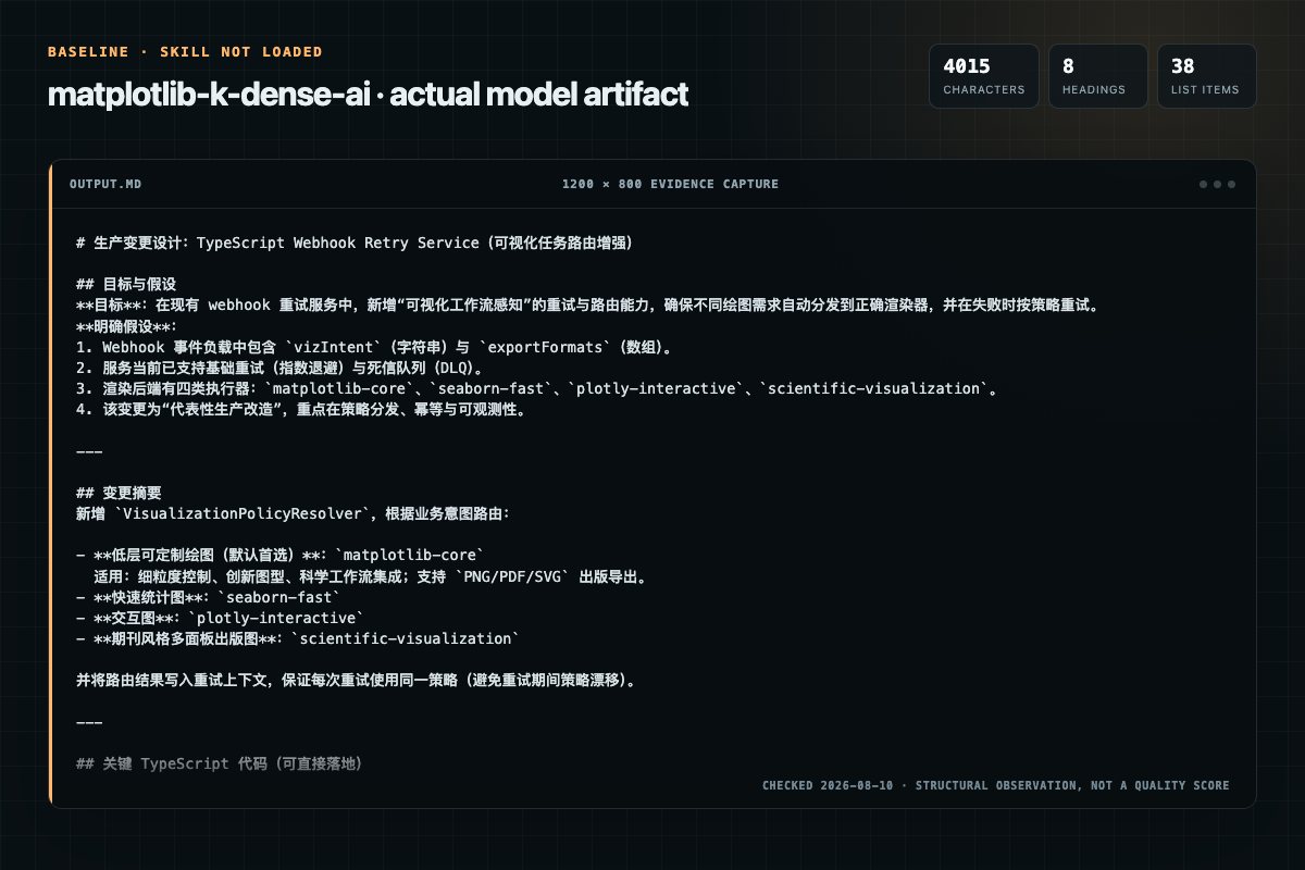
Baseline: 4015 non-whitespace characters, 8 headings, and 38 list items.
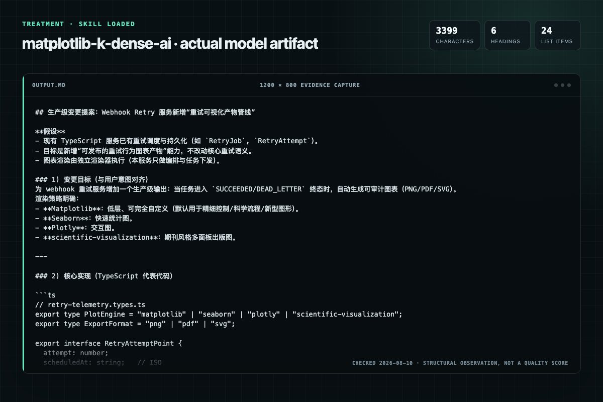
With Skill: 3399 non-whitespace characters, 6 headings, and 24 list items.
| Observation | Without Skill | With Skill |
|---|---|---|
| Source-signal coverage | 1/8: matplotlib | 1/8: matplotlib |
| Output structure | 4015 chars · 8 headings · 38 list items · 3 code blocks | 3399 chars · 6 headings · 24 list items · 5 code blocks |
| Verification and caution signals | 13 verification signals · 5 risk/limitation signals | 9 verification signals · 3 risk/limitation signals |
Use the matplotlib Skill pinned at 390f5146bf3c for my task. Follow its source-specific constraints around `matplotlib`, `setup`, `concepts`, `hierarchy`, then return the finished deliverable with explicit assumptions, verification, failure conditions, and limits. Do not treat the Skill text as a factual source or claim that a single demonstration proves universal performance.
Compatibility matrix
| Platform | Status | Evidence | What to check |
|---|---|---|---|
| Codex | Not declared | No explicit evidence | Portability before use |
| Claude Code | Not declared | No explicit evidence | Portability before use |
| Cursor | Not declared | No explicit evidence | Portability before use |
| Gemini CLI | Not declared | No explicit evidence | Portability before use |
Installation
The source command is displayed only when detected. A safe inspection prompt is always available so your agent can explain every action before execution.
npx skills add https://github.com/K-Dense-AI/scientific-agent-skills --skill "skills/matplotlib"Inspect the Agent Skill "matplotlib" from https://github.com/K-Dense-AI/scientific-agent-skills/blob/36d8f13a1e754618794bf42f417884940077b4ae/skills/matplotlib/SKILL.md at commit 36d8f13a1e754618794bf42f417884940077b4ae. List every install step, command, network request, credential, file read/write, external action, and rollback step. Explain whether it fits my task. Do not install or execute anything until I approve.
Workflow
For project work, install Matplotlib with uv:
This skill should be used when: - Creating any type of plot or chart (line, scatter, bar, histogram, heatmap, contour, etc.) - Generating scientific or statistical visualizations - Customizing plot appearance (colors, styles, labels, legends) - Creating multi-panel figures with…
Matplotlib uses a hierarchical structure of objects:
Matplotlib uses a hierarchical structure of objects:
1. pyplot Interface (Implicit, MATLAB-style)
Permission review
No configured static risk pattern was detected
This is not proof of safety. Runtime behavior, indirect dependencies, and hidden external systems are outside the static scan.
Evidence record
| Signal | Value | Evidence type | Meaning |
|---|---|---|---|
| Quality score | 95/100 | Computed | Documentation, specificity, maintenance, and trust rules |
| Repository stars | 34,478 | Source | Repository attention, not individual Skill quality |
| Compatibility | 0 platforms | Source | Declared in the catalog source record |
| Usage guide | tested outcome page | Tested | Generated or reviewed according to the visible evidence level |
Pinned source
Matplotlib is Python's foundational visualization library for creating static, animated, and interactive plots. This skill provides guidance on using matplotlib effectively, covering both the pyplot interface (MATLAB-style) and the object-oriented API (Figure/Axes), along with best practices for creating publication-quality visualizations.
This skill should be used when:
For project work, install Matplotlib with uv:
uv add matplotlib
For notebook interactivity:
uv add matplotlib ipympl
Then enable the widget backend in Jupyter with %matplotlib widget or %matplotlib ipympl.
Matplotlib 3.10 requires Python 3.10+ and NumPy 1.23+. Non-interactive file output works through backends such as Agg, PDF, and SVG. For GUI windows, Matplotlib auto-selects an available backend; if TkAgg fails in a uv-managed Python, update uv and Python builds with uv self update and uv python upgrade --reinstall, or install a Qt backend with uv add pyside6.
Matplotlib uses a hierarchical structure of objects:
1. pyplot Interface (Implicit, MATLAB-style)
import matplotlib.pyplot as plt

plt.plot([1, 2, 3, 4])
plt.ylabel('some numbers')
plt.show()
2. Object-Oriented Interface (Explicit)
import matplotlib.pyplot as plt

fig, ax = plt.subplots()
ax.plot([1, 2, 3, 4])
ax.set_ylabel('some numbers')
plt.show()
Single plot workflow:
import matplotlib.pyplot as plt
import numpy as np

# Create figure and axes (OO interface - RECOMMENDED)
fig, ax = plt.subplots(figsize=(10, 6))

# Generate and plot data
x = np.linspace(0, 2*np.pi, 100)
ax.plot(x, np.sin(x), label='sin(x)')
ax.plot(x, np.cos(x), label='cos(x)')

# Customize
ax.set_xlabel('x')
ax.set_ylabel('y')
ax.set_title('Trigonometric Functions')
ax.legend()
ax.grid(True, alpha=0.3)

# Save and/or display
fig.savefig('plot.png', dpi=300, bbox_inches='tight')
plt.show()
Creating subplot layouts:
# Method 1: Regular grid
fig, axes = plt.subplots(2, 2, figsize=(12, 10))
axes[0, 0].plot(x, y1)
axes[0, 1].scatter(x, y2)
axes[1, 0].bar(categories, values)
axes[1, 1].hist(data, bins=30)

# Method 2: Mosaic layout (more flexible)
fig, axes = plt.subplot_mosaic([['left', 'right_top'],
                                 ['left', 'right_bottom']],
                                figsize=(10, 8))
axes['left'].plot(x, y)
axes['right_top'].scatter(x, y)
axes['right_bottom'].hist(data)

# Method 3: GridSpec (maximum control)
from matplotlib.gridspec import GridSpec
fig = plt.figure(figsize=(12, 8))
gs = GridSpec(3, 3, figure=fig)
ax1 = fig.add_subplot(gs[0, :])  # Top row, all columns
ax2 = fig.add_subplot(gs[1:, 0])  # Bottom two rows, first column
ax3 = fig.add_subplot(gs[1:, 1:])  # Bottom two rows, last two columns
Line plots - Time series, continuous data, trends
ax.plot(x, y, linewidth=2, linestyle='--', marker='o', color='blue')
Scatter plots - Relationships between variables, correlations
ax.scatter(x, y, s=sizes, c=colors, alpha=0.6, cmap='viridis')
Bar charts - Categorical comparisons
ax.bar(categories, values, color='steelblue', edgecolor='black')
# For horizontal bars:
ax.barh(categories, values)
Histograms - Distributions
ax.hist(data, bins=30, edgecolor='black', alpha=0.7)
Heatmaps - Matrix data, correlations
im = ax.imshow(matrix, cmap='coolwarm', aspect='auto')
plt.colorbar(im, ax=ax)
Contour plots - 3D data on 2D plane
contour = ax.contour(X, Y, Z, levels=10)
ax.clabel(contour, inline=True, fontsize=8)
Box plots - Statistical distributions
ax.boxplot([data1, data2, data3], tick_labels=['A', 'B', 'C'])
Violin plots - Distribution densities
ax.violinplot([data1, data2, data3], positions=[1, 2, 3])
For comprehensive plot type examples and variations, refer to references/plot_types.md.
Color specification methods:
'red', 'blue', 'steelblue''#FF5733'(0.1, 0.2, 0.3)cmap='viridis', cmap='plasma', cmap='coolwarm'Using style sheets:
plt.style.use('seaborn-v0_8-darkgrid')  # Apply predefined style
# Available styles: 'ggplot', 'bmh', 'fivethirtyeight', etc.
print(plt.style.available)  # List all available styles
Customizing with rcParams:
plt.rcParams['font.size'] = 12
plt.rcParams['axes.labelsize'] = 14
plt.rcParams['axes.titlesize'] = 16
plt.rcParams['xtick.labelsize'] = 10
plt.rcParams['ytick.labelsize'] = 10
plt.rcParams['legend.fontsize'] = 12
plt.rcParams['figure.titlesize'] = 18
Text and annotations:
ax.text(x, y, 'annotation', fontsize=12, ha='center')
ax.annotate('important point', xy=(x, y), xytext=(x+1, y+1),
            arrowprops=dict(arrowstyle='->', color='red'))
For detailed styling options and colormap guidelines, see references/styling_guide.md.
Export to various formats:
# High-resolution PNG for presentations/papers
fig.savefig('figure.png', dpi=300, bbox_inches='tight', facecolor='white')

# Vector format for publications (scalable)
fig.savefig('figure.pdf', bbox_inches='tight')
fig.savefig('figure.svg', bbox_inches='tight')

# Transparent background
fig.savefig('figure.png', dpi=300, bbox_inches='tight', transparent=True)
Important parameters:
dpi: Resolution (300 for publications, 150 for web, 72 for screen)bbox_inches='tight': Removes excess whitespacefacecolor='white': Ensures white background (useful for transparent themes)transparent=True: Transparent backgroundfig = plt.figure(figsize=(10, 8))
ax = fig.add_subplot(111, projection='3d')
# Surface plot
ax.plot_surface(X, Y, Z, cmap='viridis')
# 3D scatter
ax.scatter(x, y, z, c=colors, marker='o')
# 3D line plot
ax.plot(x, y, z, linewidth=2)
# Labels
ax.set_xlabel('X Label')
ax.set_ylabel('Y Label')
ax.set_zlabel('Z Label')
fig, ax = plt.subplots(figsize=(10, 6))constrained_layout=True or tight_layout() to prevent overlapping elementsfig, ax = plt.subplots(constrained_layout=True) is recommended for automatic spacingrasterized=True in plot calls to reduce file size# Good practice: Clear structure
def create_analysis_plot(data, title):
"""Create standardized analysis plot."""
fig, ax = plt.subplots(figsize=(10, 6), constrained_layout=True)
# Plot data
ax.plot(data['x'], data['y'], linewidth=2)
# Customize
ax.set_xlabel('X Axis Label', fontsize=12)
ax.set_ylabel('Y Axis Label', fontsize=12)
ax.set_title(title, fontsize=14, fontweight='bold')
ax.grid(True, alpha=0.3)
return fig, ax
# Use the function
fig, ax = create_analysis_plot(my_data, 'My Analysis')
fig.savefig('analysis.png', dpi=300, bbox_inches='tight')
This skill includes helper scripts in the scripts/ directory:
plot_template.pyTemplate script demonstrating various plot types with best practices. Use this as a starting point for creating new visualizations.
Usage:
uv run python scripts/plot_template.py
style_configurator.pyInteractive utility to configure matplotlib style preferences and generate custom style sheets.
Usage:
uv run python scripts/style_configurator.py
For comprehensive information, consult the reference documents:
references/plot_types.md - Complete catalog of plot types with code examples and use casesreferences/styling_guide.md - Detailed styling options, colormaps, and customizationreferences/api_reference.md - Core classes and methods referencereferences/common_issues.md - Troubleshooting guide for common problemsMatplotlib integrates well with:
%matplotlib inline or %matplotlib widgetconstrained_layout=True or tight_layout()plt.close(fig)plt.rcParams['font.sans-serif']pixels = dpi * inchesFrequently asked questions
Low-level plotting library for full customization. Export to PNG/PDF/SVG for publication.
The source record exposes this install command: npx skills add https://github.com/K-Dense-AI/scientific-agent-skills --skill "skills/matplotlib". Inspect the command and pinned source before running it.
Alternatives
terrylica/cc-skills
Control Notion via Python SDK. TRIGGERS - Notion API, create page, query database, add blocks.
K-Dense-AI/scientific-agent-skills
Distributed computing for larger-than-RAM pandas/NumPy workflows. Use when you need to scale existing pandas/NumPy code beyond memory or across clusters. Best for parallel file processing, distributed ML, integration with existing pandas code. For out-of-core analytics on single machine use vaex; for in-memory speed use polars.
K-Dense-AI/scientific-agent-skills
Medicinal chemistry filters for compound triage. Apply drug-likeness rules (Lipinski, Veber, CNS), structural alert catalogs (PAINS, NIBR, ChEMBL), complexity metrics, and the medchem query language for library filtering.
K-Dense-AI/scientific-agent-skills
Use NeuroKit2 to build or audit reproducible research workflows for physiological time-series preprocessing, event/interval analysis, multimodal alignment, variability, and complexity. Trigger when code imports neurokit2 or needs its current APIs, schemas, and method-aware validation—not for diagnosis or device validation.